의사결정규칙을 나무구조와 같이 도표화하여 분류와 예측작업을 수행하는 분석 방법입니다. 여러 가지 규칙을 순차적으로 적용하면서 독립 변수 공간을 분할하는 분류모형입니다.

의사결정나무의 구성요소
- 뿌리마디(root node) : 시작되는 마디로 전체 자료를 포함
- 자식마디(child node) : 하나의 마디로부터 분리되어 나가 2개 이상의 마디들
- 부모마디(parent node) : 주어진 마디의 상위 마디
- 끝마디(terminal node) : 자식마디가 없는 마디
- 중간마디(internal node) : 부모마디와 자식마디가 모두 있는 마디
- 가지(branch) : 뿌리마디로부터 끝 마디까지 연결된 마디 들
- 깊이(depth) : 가지를 이루고 있는 마디의 갯수
의사결정나무의 원리
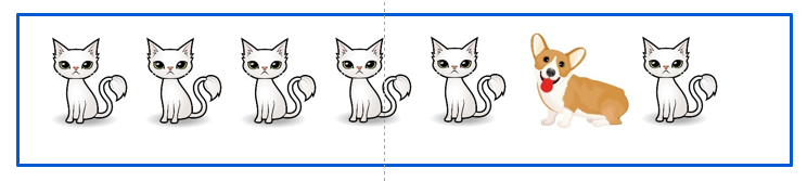
- "예"와 "아니요"로 답변하는 스무고개와 유사하다

분리기준
- 타깃변수가 범주형인 경우의 분리기준
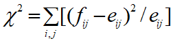
- 카이제곱 통계량 :
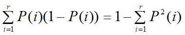
-지니계수
- 엔트로피 지수

- 타깃변수가 계량형인 경우의 분리기준
- 분산분석에서 F-통계량의 유의확률
- 분산의 감소량
- 지니계수

- 엔트로피지수

의사결정나무 알고리즘
- CART(Classification and Regression Tree(Breiman et al., 1984) : 이진분리, 지니지수, 분산의 감소량으로 분리합니다. 분류(classification)와 회귀 분석(regression)에 모두 사용될 수 있기 때문에 CART(Classification And Regression Tree)라 합니다.
- C4.5 & C5.0 : 다지분리가 가능하고, 엔트로피 지수를 사용합니다.
- CHAID (Chi-squared Automatic Interaction Detection) : 범주형 입력변수, 카이제곱검정과 분산분석의 F-검정으로 분리합니다.
의사결정나무 실습
Scikit-Learn에서 의사결정나무는 DecisionTreeClassifier 클래스로 구현되어 있습니다.
|
#의사결정나무를 위하여 iris 데이터 셑을 학습용과 검증용 데이터 셑으로 분류
from sklearn.model_selection import train_test_split
from sklearn.tree import DecisionTreeClassifier #의사결정나무 모듈 가져옴
from sklearn.datasets import load_iris
iris=load_iris()
X, y = iris.data, iris.target
X_train, X_test, y_train, y_test = train_test_split(X, y, test_size=0.3, random_state=2222) #학습용 70%, 테스트용 30% 나눔
|
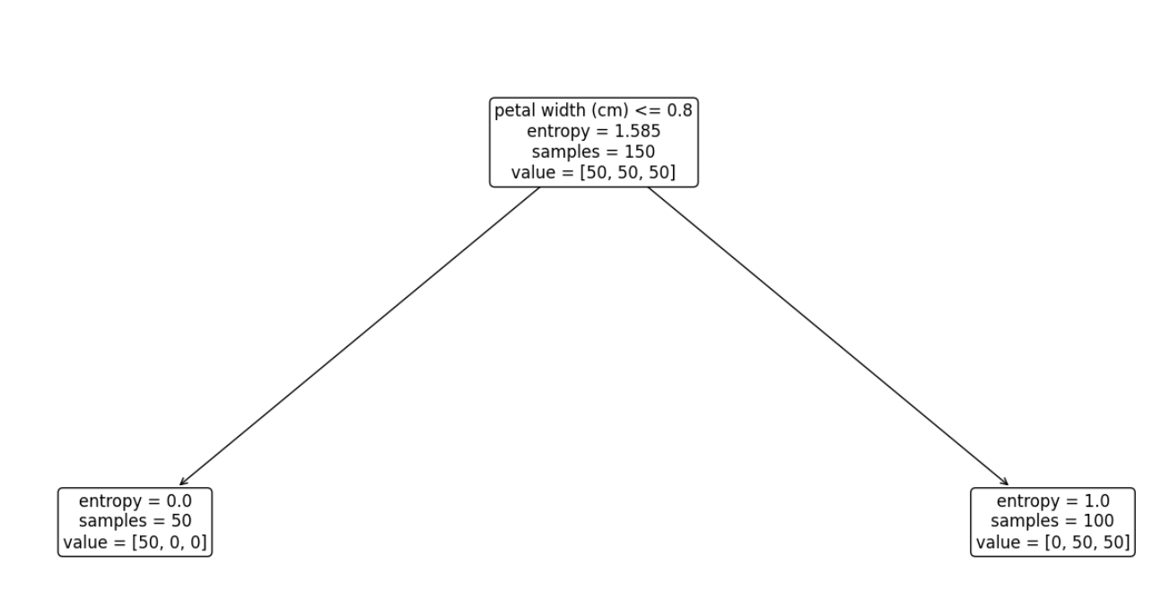
분리기준은 엔트로피 지수이고, 분리의 depth는 1로 하였고 해당하는 treee는 아래와 같습니다.
|
#분리기준 엔트로피 지수를 이용하여 의사결정나무를 작성
from sklearn.tree import DecisionTreeClassifier
dtc1 =DecisionTreeClassifier(criterion='entropy', max_depth=1, random_state=2222).fit(X, y)
plt.figure(figsize=(24,10))
plot_tree(dtc1, max_depth=1, feature_names=['sepal length (cm)', 'sepal width (cm)', 'petal length (cm)', 'petal width (cm)'], rounded=True, fontsize=12)
plt.show()
|
petal width가 0.8 이하이면 분할이 되고, 이때 setosa가 50개 중 50개가 분류되었습니다.
분리기준은 엔트로피 지수이고, 분리의 depth는 2로 하여 의사결정나무의 마디를 만들었습니다.
|
from sklearn.tree import DecisionTreeClassifier
dtc2 =DecisionTreeClassifier(criterion='entropy', max_depth=2, random_state=2222).fit(X, y)
plt.figure(figsize=(24,10))
plot_tree(dtc2, max_depth=2, feature_names=['sepal length (cm)', 'sepal width (cm)', 'petal length (cm)', 'petal width (cm)'], rounded=True, fontsize=12)
plt.show()
|
depth가 2인 경우 petal width가 1.75 이하이면 분할이 되고, 이때 versicolor 50개 중 49개, virginica 50개 중 45개 가 분류되었습니다.

분리기준은 엔트로피 지수이고, 분리의 depth는 4로 하여 의사결정나무의 마디를 만들었습니다.
|
#분리기준 엔트로피 지수를 이용하여 의사결정나무를 작성
from sklearn.tree import DecisionTreeClassifier
dtc4 =DecisionTreeClassifier(criterion='entropy', max_depth=4, random_state=2222).fit(X, y)
plt.figure(figsize=(24,10))
plot_tree(dtc4, max_depth=4, feature_names=['sepal length (cm)', 'sepal width (cm)', 'petal length (cm)', 'petal width (cm)'], rounded=True, fontsize=12)
plt.show()
|

최종 depth를 4로 두고, 학습데이터와 테스트 데이터를 나누어서 성능을 평가하도록 하겠습니다.
|
from sklearn.tree import DecisionTreeClassifier
from sklearn.model_selection import train_test_split #학습데이터와 테스트데이타를 나눔
X_train, X_test, y_train, y_test = train_test_split(X, y, test_size=0.3, random_state=2222)
dtc = DecisionTreeClassifier(criterion='entropy', max_depth=4, random_state=2222).fit(X, y)
dtc = dtc.fit(X_train,y_train)
y_pred = dtc.predict(X_test)
|
검증평가를 합니다. 정확도는 0.96이고, setosa의 f1-score는 1로 100%로 정확하고, versicolor 0.93, virginica 0.94로 평가됩니다.
|
from sklearn.metrics import confusion_matrix
from sklearn.metrics import classification_report #
print(confusion_matrix(y_test, y_pred))
print(classification_report(y_test, y_pred))
|

향후 여러 분류모델 중에 성능평가를 해서 최적의 모델을 선정해야 됩니다.
'데이터분석 > 데이터 분류 및 군집화' 카테고리의 다른 글
| Random Forest와 XGBoost(eXtreme Gradient Boosting) (0) | 2023.11.15 |
|---|---|
| 앙상블(Ensemble)의 기본개념 및 Bagging 예제 (0) | 2023.11.15 |
| 분류모형의 성능평가 (0) | 2023.10.22 |
| 중심 기반 군집의 K-Means 군집화 알고리즘 (0) | 2023.10.06 |
| 데이터 계층적 군집화(Hierarchical Clustering) (0) | 2023.10.04 |